Statistical Auditing Group

A confusion matrix is a table that assesses an algorithm's performance in binary classification[1]. This table is created by comparing the algorithm's predictions with the ground truth information, which is assumed to be the true classification of the items. Through this comparison, we obtain the number of correct and incorrect predictions made by the algorithm for both the positive and negative classes.

A classification algorithm produces a correct classification when the class assigned to an item by the algorithm (the predicted value) matches the class assigned to the item based on ground truth information. Conversely, AI produces an incorrect classification when these two values do not match. An incorrect classification is called a classification error. Classification errors occur when an algorithm misclassifies an item, "confusing" the correct and true classification with the incorrect one. This is why the table is referred to as a confusion matrix.

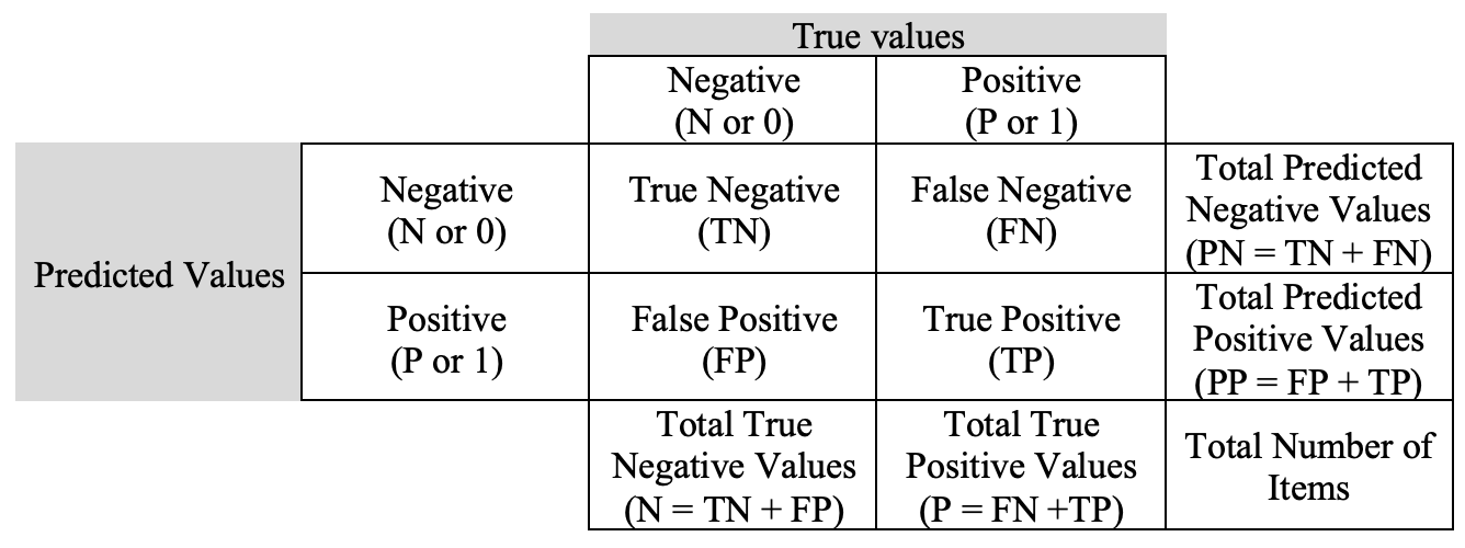
Different labels are used to denote the possible correct classifications and incorrect classifications:

1. True positive: The number of items where the algorithm's predicted positive classification matches the true positive classification
2. True negative: The number of items where the algorithm's predicted negative classification matches the true negative classification
3. False positive: The number of items where the algorithm's predicted positive classification does not match the true negative classification
4. False negative: The number of items where the algorithm's predicted negative classification does not match the true positive classification

The algorithm's predictive performance is evaluated by combining these elements of the confusion matrix in the so-called Model evaluation metrics. Model evaluation metrics are quantitative measures that assess the quality of the predictions made by the algorithm based on specific aspects, using elements from the confusion matrix that are combined in their formulas.

We can use JASP to provide an example of a confusion matrix. In the Regression section of the Data Library there is the Titanic dataset. In this example, the goal is to predict the survival of Titanic passengers. The dataset includes the ground truth information regarding the passengers' survival, represented by the binary variable Survived. This variable takes the value 0 if the passenger died and the value 1 if the passenger survived. The value 0 corresponds to the negative class, while the value 1 corresponds to the positive class. A logistic regression model has been applied to predict the passengers' survival, meaning to obtain a binary classification of the passenger in the two possible class (died or survived). After obtaining the predictions, as mentioned earlier, a confusion matrix can be constructed by comparing these predictions with the ground truth information.

The table shown is obtained by selecting the Confusion Matrix option from the Performance Diagnostics category in the Statistics section of JASP. We can see how:

1. The true positive are equal to 158, meaning that 158 passengers are correctly classified as positive (i.e. as survived passengers) by the logistic model. In other words, the algorithm's positive classification matches the true positive classification of the passengers.
2. The true negatives are 350, meaning that 350 passengers are correctly classified as negative (i.e. as dead passengers) by the logistic model. In other words, the algorithm's negative classification matches the true negative classification of the passengers.
3. The false positive are equal 93, meaning that 93 passengers are incorrectly classified as positive by the logistic model (i.e. as survived passengers). In other words, the algorithm's positive classification does not match the true negative classification of the passengers.
4. The false negative are equal to 155, meaning that 155 passengers are incorrectly classified as negative by the logistic model (i.e. as dead passengers). In other words, the algorithm's negative classification matches the true positive classification of the passengers.

Footnotes

[1] In machine learning, an algorithm that performs binary classification classifies items into one of two classes (the positive class and the negative class). This type of algorithm is known as a binary classifier.

This is an English translation of our post on the Dutch website accountant.nl.

This is the third and final post in a series of columns on machine learning in auditing. The goal of machine learning is to make predictions from data. Three main applications are typically distinguished within this field: classification, regression and clustering. Post #7 looked at classification and post #8 looked at regression. This post is about clustering.

The three main applications of machine learning can be divided into two categories: supervised learning and unsupervised learning. Which main application belongs to which category is indicated by a check mark in the table below.

	Classifcation	Regression	Clustering
Supervised learning	✓	✓
Unsupervised learning			✓

Supervised learning involves providing an algorithm with certain features and the corresponding outcome, with the goal that the algorithm learns the relationship between these features and the outcome. Classification and regression are typical examples. The first column discusses a classification algorithm, which predicts, based on customer features, whether a customer will cancel a contract in the coming year. Similarly, the second column deals with a regression algorithm, which predicts the selling price of a home based on building features. These algorithms are thus used to learn the relationship between the features and the outcome, and then use them to make predictions. You can use the information derived from these predictions to further design the audit.

In addition to supervised learning, there is also unsupervised learning. This is a form of machine learning where you have an algorithm discover patterns in data without a specific outcome variable. Clustering is a form of unsupervised learning. The goal of clustering is to discover group structure in the data based on some numerical and/or categorical features. You can usefully apply this technique in an audit. For example, you can use clustering to group customers of an online platform based on different features such as purchasing behavior, demographics and interactions with company services. This can help identify risks for specific customer segments. In addition, you can use clustering, for example, at a financial institution to identify account holders who exhibit a different combination of features. For example, a different combination of age, the number of cash withdrawals or deposits and the number of foreign transactions. These account holders can then be investigated for unusual transactions and possible fraud.

In this post, we demonstrate how to use the free open-source statistics program JASP (JASP Team, 2024; www.jasp-stats.org) without any programming knowledge to apply a machine learning algorithm for clustering in the context of an audit. We illustrate this using an example where, as an auditor, you want to cluster business locations of a storage facility landlord based on a number of features.

Imagine you are conducting an audit for a company that is in the business of renting out storage units spread across various locations throughout the country. As part of this audit, you want to check the reported sales of the company's locations for accuracy. In order to be able to make a statement on this with a degree of certainty, you want to apply a random sample. This involves visiting a selection of random business locations to check the records. By clustering the business locations, you can better organize your audit work by focusing on the business locations with the highest risks. For example, you can take a relatively small sample in the business locations that have a low risk of administrative errors and a relatively larger one in the high-risk locations. In this way, you can use your time and staff more efficiently.

To make the example concrete, we use-a slightly edited version for this post of-the publicly available Pistil Storage dataset[1]. The data contains features of 1531 business locations of the storage landlord, including reported revenue, number of available storage units, and number of FTEs working on administration[2]. You want to apply stratification in the audit of the storage landlord by using an algorithm to cluster the business locations based on these features.

Stratification

Stratification involves dividing a population into subpopulations, also called strata (Touw & Hoogduin, 2012, p. 219). This is useful when sampling from a heterogeneous population. Indeed, by dividing a population with a relatively large spread in errors into strata with a smaller spread, you can make a more accurate estimate of error for a given sample size. Conversely, this means that you can achieve the desired certainty with a smaller sample than if you did not stratify. In such situations, this allows you to reach a decision earlier, such as approval, which increases the efficiency of the sampling process.

Thus, with a stratified sample, it is necessary to divide the population into different strata that are internally similar but different from each other. So in the context of the example, you would want to divide business locations that are very similar into the same strata, while you would want to divide business locations that are very different from each other into different strata. This can be done in a rule-based way based on features of the business locations, such as turnover. To do this in a data-driven way, you can use a clustering algorithm.

Clustering

A clustering algorithm is based on the idea that some group structure can be discovered in the features of business locations. These algorithms function by exploring the data space and identifying groups, or "clusters", of business locations that have similar combinations of features. Exactly what is considered "similar" depends on the specific clustering algorithm you use. For example, clustering can be based on the distance between features in a multidimensional space, or on the density of features in this space.

Although the methodology may differ, the outcome of a clustering algorithm is always similar: a set of clusters within which the business locations have combinations of features that are more similar to each other than to the combinations of features of business locations in other clusters. It is important to emphasize here that clustering has a different purpose than classification. Indeed, you are not looking for a "correct" number of clusters in this context. In practice, you want to try different options and look for the most useful or best interpretable group classification.

Thus, although a clustering algorithm identifies a number of clusters, it is up to the auditor to determine whether these clusters are interpretable and whether meaning can be assigned to them. In the next section, we first discuss how the auditor can statistically identify and interpret clusters. In the section after that, we discuss the business interpretation of the clusters.

Applying a clustering algorithm

Applying a clustering algorithm can be done in JASP by first downloading JASP from www.jasp-stats.org and installing it. After loading the data into JASP, you can enable the Machine Learning module by clicking on the "+" symbol in the upper right corner and selecting "Machine Learning". This will make the module appear in the menu at the top of the screen. By then clicking on the module, you can see all the functionalities the module offers. In addition, the menu in the top left corner (Preferences - Interface - Preferred language) allows you to set the interface and results to be displayed in your prefererd language.

As shown in the figure above, several clustering algorithms are available for identifying group structure in the features of business locations. In this post, we use a so-called random forest algorithm (James et al., 2023, pp. 346-347). This algorithm creates multiple decision trees, each based on a varying portion of the data, where the final assignment of business locations to clusters is determined by the majority vote of these decision trees. To use this algorithm in JASP, from the Machine Learning menu, select 'Random Forest' under 'Clustering'.

In the interface shown below, you first check the option 't-SNE cluster plot' under the heading 'Plots'. This indicates that you want the different clusters to be displayed graphically. Then you unfold the 'Training Parameters' section and select the option 'Fixed' under the heading 'Cluster Determination', so that the algorithm will determine the default filled-in number of three clusters. You can also set the number of clusters yourself here or let the algorithm determine the optimal number of clusters. In this section, also check the option 'Set seed'. This sets the random number generator for the cluster algorithm to the value of 1, so that the results are reproducible on your own computer. Next, drag all features except Locatie into the 'Features' box.

Once all the data are entered, JASP starts applying the clustering algorithm. The results are shown below. The top table provides insight into the inputs to the algorithm, such as the number of clusters we had the algorithm determine (3) and the total number of data points (1531). In addition, it shows statistics that say something about the quality of the algorithm's output, such as the coefficient of determination R². It was explained in the previous column on regression that this value is a measure of the explained variance of a statistical model. In a clustering context, an R² value of 0.541 means that the clustering model can explain 54.1 percent of the total variance in the data. In other words, the clusters formed by the model explain about 54.1 percent of the dispersion in the data points around the cluster averages. You can use the remaining statistics (AIC, BIC and silhouette score) to compare models with a different number of clusters. For convenience, we won't go into that in this post, but work with a fixed number of clusters.

The second table in the output shows information about the clusters. This cluster information table shows that 499 of the 1531 sites in the dataset are assigned to the first cluster, while 543 and 489 sites are assigned to the second and third clusters, respectively. In the second and third lines of the table, you can read the within sum of squares in both percentages and absolute numbers. The within sum of squares is a measure that indicates the distribution of data within each cluster. If you express this value as a percentage of the total variance in the data, you get the explained proportion of within-cluster heterogeneity. This measure ranges from 0 to 1 and can be useful for understanding the relative importance or "weight" of each cluster. A high value of the explained proportion of within-cluster heterogeneity indicates a cluster with a lot of variance, possibly due to a large number of data points or a large spread of data points, while a low value indicates a more compact cluster. In this case, the second cluster explains about forty percent of the total explained variance, while the first and third clusters each explain about thirty percent of the total variance.

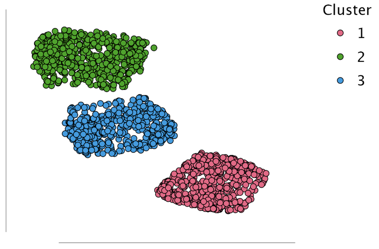
The final element in the output is a two-dimensional representation of the features of the business locations, known as the t-SNE cluster graph. The t-SNE algorithm is designed to project business locations, which are similar based on their features, to points that are close together in two-dimensional space. At the same time, business locations, which are very different in their features, are projected to points further apart in this two-dimensional space. This visualization can be useful in determining how many clusters you could create when partitioning the data. For example, the t-SNE graph below shows three distinguishable groups of business locations that are very similar. This indicates that the three clusters we had the algorithm determine are a good representation of the group structure in the data.

Once you are satisfied with the results of the algorithm, the next step is to add the cluster determinations to the data. You do that by clicking the "Add predictions to data" option in the interface and entering Cluster as the column name. That will cause the results of the cluster algorithm to be added to the data in a new column.

Interpretation

With the results of the clustering algorithm, you can perform follow-up analysis to interpret the clusters in business terms. You can do this, for example, by calculating descriptive statistics of the attributes for each cluster. To do this, go to 'Descriptive statistics' and drag all the attributes, except Locatie, to the field for 'Variables'. Then you drag the variable Cluster to the field for 'Split'. Finally, in the expandable 'Customizable Plots' section, you can check the 'Boxplots' option.

In the first two figures, you can see that the business locations in the first cluster are distinguished by relatively low turnover ('omzet' in Dutch) and low number of storage units ('eenheden' in Dutch), while the business locations in the second cluster have relatively high turnover and many storage units. The third cluster is somewhere in between these two. This suggests that the grouping of business locations is explained by the size of the locations[3]. It is interesting to note that although the business locations in three clusters differ in size, on average they have the same number of FTEs working on administration.

You can use these results to estimate the risk of misstatements in reported turnover for each cluster. For example, you could argue that the first cluster has a relatively low risk of misstatements in the administration because the business locations in this cluster with an average number of FTEs are responsible for the administration of a lower turnover. Conversely, one could argue that the second cluster has a relatively high risk of misstatements in administration because it has to account for higher turnover with the same number of FTEs. The third cluster is somewhere in between these two, and you could therefore estimate the risk of misstatements in administration as average for this cluster.

Actions

Based on the results of this analysis, you can perform a stratified sample. Here you consider the clusters as strata with different risk profiles. This allows you to consider taking a relatively large sample from business locations assigned to the stratum with a high risk of misstatements in reported turnover. At the same time, you can take a relatively small sample from business locations assigned to the stratum with a low risk of misstatements in reported turnover. This approach makes for an efficient sampling strategy, because it means you are likely to have to do less work than if you had not used stratification.

Of course, you can also use this workflow in JASP to apply a cluster algorithm for other auditing purposes. If you want to use these techniques yourself, you can download and install JASP for free at www.jasp-stats.org.

Footnotes

[1] The original dataset can be found at https://publications.aaahq.org/cia/article-supplement/7048/zip/ciia-15-1-spistil/.

[2] These data can be found at https://www.statisticalauditing.com/files/resources/data_storage.csv.

[3] By clicking on the "Feature importance" option in the cluster algorithm interface, you can have the algorithm determine which features are most dominant in forming the clusters. In this case, they are revenue, ad budget and number of storage units, all of which are positively related to the size of the business location.

References

JASP Team. (2024). JASP (Version 0.19.1) [Computer software].

James, G., Witten, D., Hastie, T., Tibshirani, R., & Taylor, J. (2023). An Introduction to Statistical Learning with Applications in Python. Springer. https://hastie.su.domains/ISLP/ISLP_website.pdf.download.html

Touw, P., & Hoogduin, L. (2012). Statistiek voor Audit en Controlling. Boom uitgevers Amsterdam.

One can quite easily come up with a simplified expression for the impartial Bayes factor if there are no misstatements discovered in the sample (i.e., k = 0). This expression is \(BF_{10} = \frac{2}{(1 - \theta_{max})^n} - 1\), where \(n\) is the sample size and \(\theta_{max}\) is the performance materiality as a percentage. I'll leave it up to the interested reader to determine the steps involved.

For example, for a performance materiality of 3 percent and a sample size of 40 items, the Bayes factor in favor of tolerable misstatement is \(BF_{10} = \frac{2}{(1 - 0.03)^{40}} - 1\) = 5.763331. We can verify this using the jfa package.

R code

By extension, this means that the required sample size to achieve a Bayes factor \(BF_{10}\) is equal to \(n = \lceil\frac{\ln(\frac{2}{1 + BF_{10}})}{\ln(1 - \theta_{max})}\rceil\). So, to achieve a Bayes factor \(BF_{10} = 19\) when expecting no misstatements, one must audit a sample of size \(n = \lceil\frac{\ln(\frac{2}{1 + 19})}{\ln(1 - 0.03)}\rceil\) = 76. Again, we can verify this using the jfa package.

R code

The Bayes factor threshold can also be formulated in terms of \(\alpha\), the sampling risk to incorrectly conclude that a population is free of material misstatement (Mensink et al., 2024). At a required Bayes factor threshold of \(BF_{10} = \frac{1-\alpha}{\alpha}\), the Bayesian required sample size reduces to \(n = \lceil\frac{\ln(2\alpha)}{\ln(1-\theta_{max})}\rceil\). Interestingly, the required sample size for a classical procedure is equal to \(n = \lceil\frac{\ln(\alpha)}{\ln(1 - \theta_{max})}\rceil\). This means that, for any level of \(\alpha\), the ratio of Bayesian sample size compared to classical sample size is \(\frac{\ln(2\alpha)}{\ln(1-\theta_{max})} / \frac{\ln(\alpha)}{\ln(1-\theta_{max})}\) = \(\frac{\ln(2\alpha)}{\ln(\alpha)}\). Consequently, the reduction in sample size is \(1 - \frac{\ln(2\alpha)}{\ln(\alpha)}\) = \(-\frac{\ln(2)}{\ln(\alpha)}\). For example, for \(\alpha\) = 0.05 the percentual reduction is 23.24 percent and for \(\alpha\) = 0.01 the percentual reduction is 15.05 percent. Plotting this relationship gives the following figure.

References

Mensink, L., de Swart, J., Derks, K., & Wetzels, R. (2024). Enhancing Efficiency and Flexibility in Audits through Bayesian Optional Stopping. PsyArXiv.

In our preprint on the impartial prior distribution, we highlight that a traditional frequentist analysis (excluding the audit risk model) is analogous to a Bayesian analysis using an improper beta(1, 0) prior distribution (first image). For those familiar with this blog, this prior may resemble the uniform beta(1,1) prior distribution (second image). However, while the uniform prior is evenly spread across all possible values of the misstatement, the improper beta(1, 0) prior concentrates all probability mass (infinitely so) at the value 1.

This implies that the improper beta(1, 0) prior assumes the population is fully misstated, with no other possibilities. In hypothesis testing, this means the probability mass to the right of the performance materiality is always 100 percent. Consequently, the auditor expresses the opinion that there is a 100 percent risk of material misstatement. This scenario is familiar to auditors who use the audit risk model with all risks set to ‘high,’ often chosen in the absence of specific risk information. Setting all risks to ‘high’ also implies a 100 percent risk of material misstatement. Thus, the equivalence between these two approaches is rooted in intuition.

Now, the question arises: is this a reasonable assumption to make? Why would you audit the population if you are already certain that a material misstatement exists? Naturally, a high risk of material misstatement leads to a larger sample size. How can you justify this to the auditee, who bears the audit costs?

The impartial prior distribution (last image) assumes that material misstatement is as likely as non-material misstatement a priori. In audit risk model terms, this equates to a 50 percent risk of material misstatement. This provides a fair starting point in the absence of specific information about the risk, rather than assuming a 100 percent risk.

Using the impartial prior can reduce the sample size by up to 23 percent compared to a traditional approach. For example, if the traditional frequentist approach suggests a sample size of 59 monetary units, using the impartial prior would result in a sample size of 45 units. Are we auditing too much?

While the auditing standards, such as the International Standards on Auditing (ISA), do not mandate the use of a specific statistical framework (i.e., frequentism or Bayesianism) when performing an audit, sometimes I get a question about how Bayesian inference fits within these standards. My answer is that the auditing standards not only seem to approve of Bayesian inference but probably align better with Bayesian methods than with frequentist statistics.

Trevor Stewart's 2013 thesis on Bayesian inference in auditing (Stewart, 2013) includes a subchapter (Chapter 2.2), discussing why auditors are essentially Bayesians. While I won't reproduce his full text here, it is an interesting read, and you can access it via this link.

Stewart tells us that auditing standards inherently describe the audit process as Bayesian. For example, he notes that these standards state, "an audit of financial statements is a cumulative and iterative process" (ISA 330, paragraph A62). This, of course, aligns well with the Bayesian philosophy of updating information (Derks et al., 2021).

Although the above quote from the ISA is the only direct quote that Stewart uses, there are other instances where the standards implicitly suggest that the audit is Bayesian. For instance, they also state, "The auditor's risk identification and assessment process is iterative and dynamic" (ISA 315, paragraph 7), and "Obtaining an understanding of the entity and its environment, the applicable financial reporting framework, and the entity's system of internal control is a dynamic and iterative process of gathering, updating, and analyzing information and continues throughout the audit" (ISA 315, paragraph A48).

Moreover, audit evidence is described as "cumulative in nature" and includes "information that supports and corroborates management's assertions, and any information that contradicts such assertions" (ISA 200, paragraph A31), which aligns with the philosophy of the Bayes factor (Derks et al., 2024).

Additionally, the standards mention that "Planning is not a discrete phase of an audit, but rather a continual and iterative process" (ISA 300, paragraph A2). This suggests that the audit standards would advocate for Bayesian sequential sampling (Mensink et al., 2024), instead of the rigid sequential sampling plans required by the frequentist framework.

Regarding sample size extension, the standards note, "For example, in the case of tests of controls, the auditor might extend the sample size, test an alternative control, or modify related substantive procedures" (ISA 530, paragraph A23). This approach resembles using the posterior distribution as a prior distribution for updating via further audit activities.

In sum, I think the auditing standards should have no issue with the use of Bayesian inference.

References

Derks, K., de Swart, J., van Batenburg, P., Wagenmakers, E. J., & Wetzels, R. (2021). Priors in a Bayesian audit: How integration of existing information into the prior distribution can improve audit transparency and efficiency. International Journal of Auditing, 25(3), 621-636.

Derks, K., de Swart, J., Wagenmakers, E. J., & Wetzels, R. (2024). The Bayesian approach to audit evidence: Quantifying statistical evidence using the Bayes factor. Auditing: A Journal of Practice & Theory, 1-17.

Mensink, L., de Swart, J., Derks, K., & Wetzels, R. (2024). Enhancing Efficiency and Flexibility in Audits through Bayesian Optional Stopping. PsyArXiv.

Stewart, T. R. (2013). A Bayesian Audit Assurance Model with Application to the Component Materiality Problem in Group Audits. [PhD-Thesis - Research external, graduation internal, Vrije Universiteit Amsterdam].

Banks need a rule to make decisions regarding their clients' loan applications. These decisions are typically based on the applicants' demographic and socio-economic profiles, which loan managers must consider beforehand. An algorithm can be used to classify customers as either bad or good credit risks. This classification will influence the loan approval process.

The German Credit Risk Dataset contains information about a bank's clients. The dataset consists of 700 instances of creditworthy applicants and 300 instances of bad credit applicants. Additionally, 20 different attributes related to the bank's customer characteristics are collected. The German Credit Risk dataset is a public domain dataset available in the data repository of the UCI (University of California, Irvine). I decided to analyze the version of the dataset included in the fairness R package. For credit rating processes, certain socio-economic information about clients may be considered sensitive attributes, as their use could lead to discrimination against specific social groups. For illustrative purposes, I decided to use solely the clients' gender as the sensitive attribute. Gender is a categorical variable with two levels: male and female. These levels identify the privileged group (males) and the underprivileged group (females).

I simulated the credit risk prediction process using all the information within the dataset[1]. I obtained the predictions by applying the Boosting model with interaction (using the misclassification error, it is selected as the best model for its performance on the training set, which constituted 75 percent of the entire dataset) to the validation set (which constituted the remaining 25 percent of the dataset). By comparing the predictions with the actual information regarding clients' defaults, contained in the test set, it is possible to obtain the confusion matrices for the male (left figure) and female (right figure) groups.

To assess the presence of potential discrimination against the unprivileged group, it is necessary to use a fairness measure. I decided to use the false negative rate parity as a fairness measure[2]. I calculated the value of the false negative rate for both the privileged and the unprivileged group. For male costumers, the false negative rate is equal to 0.343, while for female costumers, the false negative rate is equal to 0.533. Women clients applying for a loan are incorrectly classified as being a bad credit risk when they are actually a good credit risk a greater number of times compared to men. It appears that the group identified as underprivileged is not being favored by the use of this algorithm.

We must verify that the observed difference is significantly different from zero to have a conclusion of our analysis. I decided to apply the two-proportion test.

R code

I use a significance level of 5 percent and obtain a statistical test p-value equal to 0.006, lower than the selected significance level. I conclude that there is strong evidence against the null hypothesis of equal false negative rates between the two groups. The significant difference between the values indicates that the algorithm causes discriminatory acts against woman because the bank will not wrongly give them the approval for the loan a greater number of times compared to men.

Footnotes

[1] A description of all the available variables can be found at https://archive.ics.uci.edu/dataset/144/statlog+german+credit+data

[2] According to the dataset description, false negatives result in greater financial losses for the bank, as granting a loan to someone who defaults causes major economic damage. In my simulation, I focused on minimizing these classification errors during the algorithm audit.

During first week of July, part of the Statistical Auditing Group went to the International Society for Bayesian Analysis (ISBA) World Meeting.

The ISBA World Meeting brings together a global community of researchers and professionals who develop and apply Bayesian methods to tackle complex problems across various fields, including economics, finance, industry, biostatistics, environmental statistics, and more. It was an inspiring week full of interesting sessions.

To give you an idea about the topics that were discussed, we created a word cloud from our notes. This visual representation captures many of the topics that were covered.

In posts #5 and #6, I delved into the methods of computing the audit sampling Bayes factor both analytically and using the Stan software. Despite the calculations not being overly complicated, they do require a substantial amount of R code. To simplify this process, you can use the jfa R package. We created this package specifically to facilitate statistical auditing.

The codeblock below shows R code to reproduce the Bayes factor calculation from post #5 and #6. It uses the evaluation() function from the package. In this function, x represents the number of misstatements in the sample (0), while n represents the number of sample items (60). As you can see from the value of BF\(_{10}\) in the output, this code accurately reproduces the Bayes factor of 32.4 in favor of tolerable misstatement.

R code

This is an English translation of my post on the Dutch website accountant.nl.

The goal of machine learning is to make predictions based on data. Within this field, three main applications are generally distinguished: classification, regression, and clustering. Post #7 dealt with classification. This post is about regression. Regression is a form of machine learning, with which you can predict a numerical outcome based on a number of features (i.e., characteristics). In an audit, for example, you can use this to predict the daily turnover of a store based on the number of customers and the location of the store, or to predict wage costs based on the number of employees and the hours worked. In this way, you can estimate whether the reported amounts of money correspond to realistic expectations.

During your education to become an accountant, you learn about linear regression, but machine learning offers the possibility to model more complex relationships as well. In this post, I will use the so-called boosting algorithm as an example, although there are numerous other algorithms available.

It is important to emphasize that the use of machine learning techniques is not so much a goal in itself. It offers you the flexibility to not be limited to one technique and to compare the results of different techniques, such as boosting and linear regression. In this way, you can select the technique that performs best in a trade-off between quality and explainability.

In this post, I show how you can train a machine learning algorithm for regression with the free open-source statistics program JASP (JASP Team, 2024) without any programming knowledge and then apply it in the context of an audit. I illustrate this with an example where you, as an auditor, want to identify the outliers in the selling prices of houses in the portfolio of a real estate developer for a fraud investigation. Please note, this is just an example. The ultimate goal of this series of posts is to challenge you to use these techniques for your own purposes.

Real estate valuation

Sometimes, real estate developers can enter into transactions with related parties at non-market prices, to increase profits or minimize losses. If the reported selling prices are significantly higher or lower than the market value, this could be an indication of fraud.

An example of this is the overvaluation of properties to obtain loans based on false value. As an auditor, you can detect these suspicious properties as outliers in the portfolio by predicting the expected selling prices of the houses during the audit using a regression analysis. The idea is that you learn from public data what a realistic selling price is for a house with certain features, and then check whether the houses in the portfolio of the real estate developer comply with this.

In this example, I use a slightly edited version of the generally accessible Housing Prices dataset[1]. Just like in the first post, it is important to emphasize that these are example data. In practice, it is advisable to use reliable information from a public database that is representative of the market in which the real estate developer is active.

The available data contains, in addition to the selling price, a number of construction technical features for 445 houses, such as the number of habitable square meters, the number of floors, and the number of bathrooms[2]. The same features are also available for the hundred houses in the developer's portfolio[3]. You want to determine the prices at which the real estate developer can realistically sell the houses in the portfolio. If a house is valued by the real estate developer at a much too low or too high price, this could be an indication of fraud.

Trainingset and testset

The premise of a regression algorithm is that there is a relationship between the construction technical features of a house and the selling price. If you know this relationship, you can make a prediction about the price at which a house should be sold based on its features. However, it is unknown how the features relate to the selling price, so the algorithm must learn this relationship from the available data.

To learn the relationship between the selling price and the construction technical features, you can show the regression algorithm a part of the available data, for example, from 345 randomly selected houses. This part of the data, which contains both the construction technical features and the selling price, is called the training set.

To then evaluate whether the learned relationship generalizes well to houses that the algorithm has not yet seen, you can keep a so-called test set separate during the training phase. This test set consists of the remaining hundred houses in the data. Once this training and test set have been established, you can start training a regression algorithm.

Tranining a regression algorithm

After downloading and installing JASP, you can import the data. Then, you can enable the Machine Learning module by clicking on the '+'' symbol in the top right corner and choosing 'Machine Learning'. This will make the module appear in the menu at the top of the screen. By then clicking on the module, you can see all the functionality that the module offers. Through the menu in the top left corner (Preferences - Interface - Preferred language), you can also set the interface and the results to be displayed in your prefererd language.

As can be seen in the above screenshot, there are various regression algorithms available for learning the relationship between the selling price and the construction technical features. In this column, I choose the boosting algorithm (James et al., 2023, pp. 347-350). This is a technique where a number of decision trees are trained in succession. Each new decision tree in this method focuses on the errors made in the previous decision trees. This improves the predictive power of the model at each step. To use this algorithm in JASP, select the 'Boosting' option under 'Regression' in the Machine Learning menu.

Next, in the interface shown below, you open the 'Data Split Preferences' section, select the 'Testset indicator' option, and assign it the variable testSet using the dropdown menu. This ensures that the algorithm uses the previously randomly selected 345 houses to train the algorithm and the remaining hundred houses to evaluate the algorithm.

In the same section, under 'Training and Validation Data', click on 'K-fold' (James et al., 2023, pp. 206-208). This indicates that during the training phase, one fifth of the training set is used as a validation set each time, while the algorithm is trained on the remaining part of the training set. This process repeats for each of the five parts of the training set, with the aim of determining the optimal number of consecutive decision trees.

By the way, you don't necessarily have to split the training set into five parts. In the interface, you can set yourself how many parts are used. The rule here is that splitting the training set into more parts gives more accurate results, but takes more time, while splitting into fewer parts is faster, but possibly less reliable.

After setting the data split preferences, you open the 'Training Parameters' section and check the 'Set seed' option. This initializes the random number generator in the boosting algorithm with the value 1, so you can reproduce the results from this post on your own computer. Then you drag the Price variable to the target variable box. Finally, select all other variables except testSet22 and drag them to the features box.

As soon as all the data is entered, JASP starts training the regression algorithm. The resulting output is shown below. The table shows that training and optimizing the algorithm results in a model that uses 68 decision trees. In this case, of the 345 homes in the training set, 276 homes (345 \(\times\) 4/5) were used five times to train the model, and 69 homes (345 \(\times\) 1/5) were used five times to optimize/validate the model. Furthermore, the output shows that this model achieves a mean squared error (MSE) of 1.001 \(\times\) 10\(^{10}\) on the hundred houses in the test set.

Evaluating quality

The mean squared error is used to optimize a regression model and is the standard measure for evaluating its quality. Optimization in this context means searching for the number of trees that results in the lowest mean squared error. However, the interpretation of this quality measure is relatively complex. For a more intuitive evaluation of the model, you can check the 'Model Performance' option under the 'Tables' heading at the top of the interface. This will display the table below with a number of quality measures. These quality measures quantify in different ways how well the predictions of the algorithm match the actual sales prices in the test set.

The top row of the table contains the aforementioned mean squared error[5]. This indicates that the average difference between a predicted and an actual sales price in the test set, when squared, is 10,013,885,887.37. It is important to note that this is the average squared difference, not the average actual difference. The reason for this is that the algorithm's predictions can be both too high and too low, and we don't want positive and negative differences to cancel each other out. By squaring the differences between the actual and predicted sales prices, they all become positive and can be added up.

The value of the mean squared error depends on the units in which the target variable is measured. To illustrate, in this example, the sales prices for all houses are expressed in euros, which means the mean squared error is displayed in terms of squared euros. If you express the sales prices in euro cents by multiplying them by a hundred, then the predicted sales prices will also be in euro cents. In that case, the mean squared error will be expressed in squared euro cents and will be ten thousand times larger.

This dependency means that there is no general guideline that indicates when this measure demonstrates sufficient quality of the model. Although the mean squared error is not easy to interpret, I mention this measure here because it is the standard way to optimize and evaluate a regression model.

A more intuitive measure of the quality of the regression model, however, is the Mean Absolute Error (MAE). This value represents the average prediction error in the original units of the target variable, in this case, euros. A mean absolute prediction error of 55,953.056 means that when predicting the price of a random house in the test set, the prediction deviates on average by € 55,953.06 from the actual sales price.

To gain insight into the relative deviations between the predicted sales prices and the actual sales prices, you can express the absolute prediction errors as a percentage of the actual sales prices and take the average of that. This measure, known as the Mean Absolute Percentage Error (MAPE), can be found in the penultimate row of the table and amounts to 5.42 percent. This means that the predicted sales prices differ on average by 5.42 percent from the actual sales prices.

Finally, for the evaluation of the quality of the algorithm, you can look at the coefficient of determination R\(^2\) (James et al., 2023, pp. 78-80), which you might know from linear regression. This can be found in the bottom line of the table with performance metrics. It shows that the algorithm can explain 95.7 percent of the variance in the sales price through the construction technical features.

You can further optimize the algorithm by adjusting the 'Algorithmic Settings' in the interface. However, this goes too deep into the subject matter to discuss in this post as well.

Application

If you are satisfied with the performance of the algorithm, the next step is to make predictions for the sales price of the hundred houses in the real estate developer's portfolio. In JASP, you can do this by first saving the trained algorithm. You do this by checking the 'Save Trained Model' option. You can then load the data of the homes in the real estate developer's portfolio into a new session.

Next, you go to the 'Prediction' analysis in the Machine Learning menu and load the saved model. You drag the construction technical features of the houses to the designated field. Then at the bottom of the interface, click on 'Add predictions to data' and fill in Predicted as the column name. This ensures that the predicted sales prices are added to the data in a new column.

With the predicted sales prices, you can perform a more extensive analysis. You can start with a visual inspection for outliers by plotting the predicted and reported sales prices against each other in a scatter plot, as shown below[6]. The red line indicates where the predicted sales price matches the reported sales price.

Houses where the predicted sales price is lower than the reported sales price are indicated by points that lie below the red line, while houses where the predicted sales price is higher than the reported sales price are indicated by points that lie above the red line. In the figure, some houses are notable because the predicted sales price considerably differs from the reported sales price.

To identify these notable houses in the data, you can create a new column in the data that indicates the absolute difference between the predicted and reported sales prices. You do this by going to the '+'' icon, which is located to the right of the last column in the data, and clicking on it.

Next, you name this column Difference and indicate through the drag-and-drop interface that this should contain the absolute value of the Prijs column minus the Predicted column (see left image below). After that, you can, for example, create a column named Notable in which you indicate whether the absolute difference is greater than a certain amount, for example € 100,000 (see right image below).

Finally, you can go to 'Descriptive Statistics' to analyze these two new columns. For example, you can determine the number of houses that deviate by more than € 100,000 by requesting a frequency table of the Notable variable (TRUE for more than € 100,000 deviation, FALSE for less than € 100,000 deviation). This table, shown below, shows that for fourteen out of a hundred houses, the predicted sales price deviates by at least € 100,000 from the reported sales price.

Actions

Based on these results, you can determine the further course of the fraud investigation. For example, you could decide to comprehensively check the sales documents of the fourteen notable properties. This includes verifying all relevant documents, such as purchase contracts, appraisal reports, and financial transaction registers.

Of course, you can also use this workflow in JASP to train a regression algorithm for other audit purposes. If you want to apply these techniques yourself, you can download and install JASP for free from www.jasp-stats.org.

Footnotes

[1] The original dataset can be found at https://www.kaggle.com/datasets/yasserh/housing-prices-dataset

[2] The (lightly) edited version of the original dataset can be found at https://www.statisticalauditing.com/files/resources/data_housing_traintest.csv.

[3] These data can be found at https://www.statisticalauditing.com/files/resources/data_housing_prediction.csv.

[4] Note that there are a total of four types of datasets: training (276), validation (69), test (100), and application (100).

[5] The second and third rows of the table show simple transformations of the mean squared error and are therefore not discussed in the text. The second row shows the MSE(scaled), which is the mean squared error, scaled so that it falls between 0 and 1. The third row shows the root mean squared error (RMSE).

[6] This graph was created by using the 'Bayesian correlation' analysis, navigating to the 'Plot Individual Pairs' section, and then entering the variables Price and Predicted. The red line was added outside of JASP.

References

JASP Team. (2024). JASP (Version 0.18.3) [Computer software].

James, G., Witten, D., Hastie, T., Tibshirani, R., & Taylor, J. (2023). An Introduction to Statistical Learning with Applications in Python. Springer. https://hastie.su.domains/ISLP/ISLP_website.pdf.download.html

This is an English translation of my post on the Dutch website accountant.nl.

The goal of machine learning is to make predictions based on data. Within this field, three main applications are typically distinguished: classification, regression, and clustering. This column is about classification.

Classification is a form of machine learning that aims to predict a categorical (i.e., non-numeric) variable based on various features (i.e., characteristics). Classification has numerous practical applications and is also used in auditing today. For example, you can use this technique to predict the continuity of a company as worrisome or not, based on various financial ratios.

In the same way, you can predict the fraud risk of claims as high or low based on, for example, the lead time and the amount that is claimed. These predictions are possible thanks to algorithms that have been trained on data. However, training these types of algorithms is not easy and often requires programming knowledge. That is a pity, because it forms an obstacle to the wider use of these innovative methods.

In this column, I demonstrate how you can train a machine learning algorithm for classification with the free open-source statistics program JASP (JASP Team, 2024; www.jasp-stats.org) without any programming knowledge and then apply it in the context of an audit. As an example, I discuss a situation where you, as an auditor, want to predict customer churn at a telecom provider as part of risk assessment activities.

Customer churn

Customer churn is the phenomenon where customers stop using a company's services. Predicting customer churn in the coming year can be relevant in the risk assessment phase of an audit, as a volatile customer base can be a risk to the continuity of the company.

In this example, I use a slightly edited version of the generally accessible Telco Customer Churn dataset[1] for this column. It is important to note that these are example data. In practice, it is better to use historical data from the telecom provider's database.

The example data contains features for 3,738 customers such as demographic information, details of the phone and internet contract, and whether the customer has terminated the contract with the telecom provider[2]. In addition to these example data, the current customer base of the telecom provider consisting of two thousand customers is also available[3]. It is still unknown for these customers whether they will terminate the contract in the coming year.

Theory classification

Before I show you how to train a classification algorithm with JASP to predict expected customer churn, I will first briefly discuss the theory behind classification. The premise of a classification algorithm is that there is a relationship between customer features and customer churn. If you know this relationship, you can predict based on the customer features whether a customer will terminate the contract in the coming year. However, it is unknown how the customer features are related to customer churn, so the algorithm must learn this relationship from historical data.

To learn the relationship, you can show the classification algorithm a part of the historical data, for example, from 3,238 customers. This is called the so-called training set. In this example, the training set contains both the features and the churn. To then evaluate whether the learned relationship generalizes well to customers that the algorithm has not yet seen, you can keep a so-called test set, consisting of five hundred customers, separate during the training phase.

Both the training set and the test set should not be too out of balance, so that there are approximately an equal number of customers who have and have not terminated present. This is important to prevent the algorithm from having a preference for one of the two classes simply because it occurs more often in the training set. In this example, the training and test set are balanced by excluding the data of some customers, resulting in a balanced distribution of customers who have and have not terminated. Once these training and test sets are available, you can start training a classification algorithm.

Training a classification algoritm

You can train a classification algorithm in JASP by first downloading JASP from www.jasp-stats.org and installing it. After loading the data into JASP, you can enable the Machine Learning module by clicking on the '+' symbol in the top right corner and choosing 'Machine Learning'. This will make the module appear in the menu at the top of the screen. By then clicking on the module, you can see all the functions that the module offers. Through the menu in the top left corner (Preferences - Interface - Preferred language), you can also set the interface and the results to be displayed in your preferred language.

As can be seen in the screenshot above, there are various classification algorithms available for learning the relationship between customer features and customer churn. In this column, I choose a K-nearest neighbors algorithm (James et al., 2023, pp. 183-188). To use this algorithm in JASP, you select the 'K-Nearest Neighbors' option under 'Classification' in the Machine Learning menu. Then, in the interface shown below, you open the 'Data Split Preferences' section, select the 'Test set indicator' option, and assign this to the testSet variable using the dropdown menu. This ensures that the algorithm uses the pre-specified 3,238 customers to train the K-nearest neighbors algorithm and uses the remaining five hundred customers to evaluate the algorithm.

In the same section, under 'Training and validation data', you click on 'Leave-one-out' (James et al., 2023, pp. 204-206). This indicates that during the training phase, one row from the training set is used as a validation set each time, while the algorithm is trained on the rest of the training set. This process is repeated for each row in the training set with the aim of allowing the algorithm to identify the optimal number of nearest neighbors, K.

Then, you open the 'Training Parameters' section and enter 100 as the maximum number[4] under the heading 'Number of Nearest Neighbors'. Next, you drag the Churn variable to the target variable box. Finally, you select all other variables except testSet and drag them to the features box.

As soon as all the data is entered, JASP starts training the classification algorithm. The resulting output is shown below. The table and the figure below show that training and optimizing the K-nearest neighbors algorithm results in a K=67 nearest neighbors model. In addition, the output shows that this K=67 nearest neighbors model achieves an accuracy of 0.79 on the test set, which means that you can correctly predict for 79 percent of the customers in the test set whether they have terminated the contract with the telecom provider

The confusion matrix below provides more insight into the performance of the algorithm by showing how the predictions for the customers in the test set match reality. The confusion matrix shows that the algorithm correctly predicts that 215 customers would terminate the contract, and it also correctly predicts that 180 customers would not terminate the contract. This leads to an accuracy of the algorithm on the test set of (215 + 180) / 500 = 0.79, which corresponds to 79 percent.

Prediction

Based on the training set, you can make an absolute prediction for a customer in the current customer base (who is not in the training set or test set) in terms of 'Yes, this customer will terminate the contract' or 'No, this customer will not terminate the contract'. However, by using a test set, you can determine the degree of uncertainty with which this prediction is made.

For a customer in the current customer base, you can now make a nuanced prediction based on the confusion matrix, such as 'Yes, this customer will terminate the contract next year with a probability of 75.4 percent', since (215 + 70) / 215 = 0.754, or 'No, this customer will not terminate the contract next year with a probability of 83.7 percent', since (180 + 35) / 180 = 0.837. It is up to you to assess whether this degree of certainty is sufficient to base conclusions on.

Application

If you are satisfied with the performance of the algorithm, the next step is to apply this algorithm to make predictions for the two thousand customers in the current customer base of the telecom provider. In JASP, you can do this by saving the trained algorithm using the 'Save Trained Model' option. You can then load the current customer base into a new session.

First, you navigate to the 'Prediction' option in the machine learning menu and load the saved model there. You then drag the features of the customers in the current customer base to the designated field. Then, at the bottom of the interface, click on 'Add Predictions to Data'. Finally, you can go to 'Descriptive Statistics' to generate frequency tables of the predictions.

This table, shown below, shows that for 120 of the two thousand current customers, or 6 percent of the current customer base, it is predicted that they will terminate the contract next year. You can further refine these predictions by taking into account the uncertainty from the test set, or by incorporating the uncertainty in the individual customer predictions. For convenience, refining the predictions is skipped in this post.

Actions

Based on the predicted customer churn, you can take actions to assess the risks to continuity. With 6 percent of the current customers expected to terminate the contract next year, there could be a significant risk of loss of income, for example, if this is not compensated with a comparable percentage of new customers. If that is indeed not the case, you can recommend taking preventive measures based on these results, such as improving customer service, offering loyalty programs, or revising pricing.

In addition, you can perform an in-depth analysis of the customers who are likely to terminate the contract to identify common features. JASP can identify the features that contribute most to the prediction. You can then use these features as a basis for your recommendations. In this case, these are, for example, the duration of the customer relationship, the type of contract (one-year, two-year, or monthly cancellable), and the use of technical support by the customer. The telecom provider can then use this information to develop targeted retention strategies and thus reduce the risk of customer churn.

Of course, you can also use this workflow in JASP to train a classification algorithm for other audit purposes. If you want to apply these techniques yourself, you can download and install JASP for free via www.jasp-stats.org.

Footnotes

[1] The original dataset can be found at https://www.kaggle.com/datasets/blastchar/telco-customer-churn.

[2] The example data used can be found at https://www.statisticalauditing.com/files/resources/data_churn_traintest.csv.

[3] These data can be found at https://www.statisticalauditing.com/files/resources/data_churn_prediction.csv.

[4] In this example, the training phase is used to determine the best value for 'K'. However, in JASP you have the option to enter a value of 'K' yourself by selecting the 'Fixed' option under 'Number of Nearest Neighbors' and entering the desired value of 'K' in the corresponding field. In that case, there is no training phase.

References

JASP Team. (2024). JASP (Version 0.18.3) [Computer software].

James, G., Witten, D., Hastie, T., Tibshirani, R., & Taylor, J. (2023). An Introduction to Statistical Learning with Applications in Python. Springer. https://hastie.su.domains/ISLP/ISLP_website.pdf.download.html

In the previous post I showed how to use Bayes' rule to calculate the audit sampling Bayes factor as the change from the prior odds to the posterior odds. However, you can also calculate the Bayes factor directly as the ratio of two marginal likelihoods. For this, you will need the rstan R package to perform sampling from the models and the bridgesampling R package to compute the log marginal likelihood of the two models.

The R code in the following codeblock computes the marginal likelihood for the model for \(H_-\), in which the misstatement rate is bounded to lie between the minimum misstatement rate of 0 and the performance materiality of 0.05.

R code

The R code in the following codeblock computes the marginal likelihood for the model for \(H_+\), in which the misstatement rate is bounded to lie between the performance materiality of 0.05 and the maximum misstatement rate of 1.

R code

The Bayes factor in favor of non-material misstatement can be computed by dividing the marginal likelihoods of \(H_-\) and \(H_+\), respectively. Since the bridge_sampler function computes the log marginal likelihood, you need to take the exponents first and then perform the division.

R code

As you can see, this replicates the Bayes factor from the previous column, which was around 32. Of course, you can use this workflow to compute the Bayes factor for any prior distribution (e.g., normal) and any value of the performance materiality.

When you conduct audit sampling, the outcome is typically binary. That is, you either conclude that you have gathered sufficient evidence to conclude that the population is free of material misstatement or you conclude that you have not. The latter situation implies that additional work is required, or that a correction will be issued to the auditee (a strategy often employed by tax authorities), after which the population can still be approved. The odd thing about making this type of binary conclusion is that there are no degrees of evidence, there exists only sufficient evidence. For instance, if no misstatements are found, reviewing a sample of 100 items and reviewing a sample of 60 items both result in the conclusion that sufficient evidence is obtained to approve the population[1]. However, the larger sample should intuitively be able to provide more statistical evidence supporting the conclusion that the population is free of material misstatement than the smaller sample because more data are observed that point in that direction.

Quantifying evidence

Auditors typically do not quantify the statistical evidence presented by the data. This is because it is challenging to do so within the traditional frequentist framework. However, in the Bayesian framework, a gradual quantification of evidence is more natural. In our recently published article, The Bayesian approach to audit evidence: Quantifying statistical evidence using the Bayes factor, we discuss how to quantify this evidence using the Bayes factor for various types of data analyses. To illustrate a typical Bayes factor calculation, let's consider an example in the context of audit sampling.

Bayes' rule for hypothesis testing

In audit sampling, the Bayes factor indicates how many times more likely the data is under the hypothesis of non-material misstatement \(H_-\) versus the hypothesis of material misstatement \(H_+\). To calculate the Bayes factor, we can use Bayes' rule for hypothesis testing, which states that the posterior odds are the product of the prior odds and the relative evidence in the data. This relative evidence is also known as the Bayes factor.

$$\underbrace{\frac{p(H_- \, | \, y)}{p(H_+ \, | \, y)}}_{\text{Posterior odds}} = \underbrace{\frac{p(y \, | \, H_-)}{p(y \, | \, H_+)}}_{\text{Relative evidence}} \times \underbrace{\frac{p(H_-)}{p(H_+)}}_{\text{Prior odds}}$$

Thus, to calculate the Bayes factor you need to obtain the prior odds and the posterior odds and divide the two. Let's look step-by-step at how this can be done

Prior odds

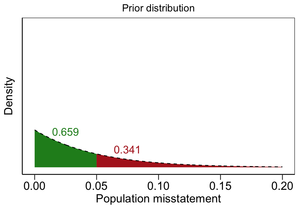
First, suppose that the auditor specifies a beta(1, 21) prior distribution based on available audit information (first image). The area under the prior distribution to the left of the performance materiality of five percent is highlighted in green. This area represents the prior probability of a non-material misstatement occurring, which is equal to \(p(H_-)\) = 0.659 (65.9 percent)[2]. The area under the prior distribution to the right of the performance materiality is the prior probability of a material misstatement occurring and is \(p(H_+)\) = 0.341 (34.1 percent). Dividing the two prior probabilities results in the so-called prior odds being \(\frac{0.659}{0.341} \approx\) 1.94 in favor of non-material misstatement.

Posterior odds

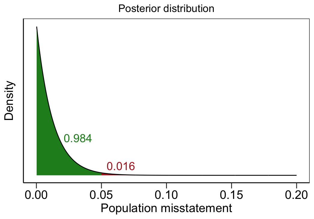
Next, suppose you obtain data \(y\) from an audited sample of 60 items not containing any misstatements. Using Bayes' rule, you can then update your beta(1, 21) prior distribution to a beta(1, 81) posterior distribution (second image) and calculate the posterior odds. The posterior probabilities are the area to the left and right of the performance materiality and roughly equal \(p(H_- \, | \, y)\) = 0.984 (98.4 percent) and \(p(H_+ \, | \, y)\) = 0.016 (1.6 percent), respectively. Dividing these posterior probabilities results in the posterior odds being \(\frac{0.984}{0.016} \approx\) 62.74.

Bayes factor

Finally, the Bayes factor can be calculated by dividing the posterior odds by the prior odds. In this case, the Bayes factor is \(\frac{62.74}{1.94} \approx\) 32.4. This means that the data are about 32 times more likely under the hypothesis of non-material misstatement than under the hypothesis of material misstatement. Now, let's see what happens to the Bayes factor if you would have reviewed a sample of 100 items with no misstatements instead. Since the prior distribution remains the same, the prior odds are still 1.933. However, using these data the posterior odds are \(\frac{0.988}{0.002} \approx\) 494. Hence, the Bayes factor is \(\frac{494}{1.94} \approx\) 255.

As you can see, using the Bayes factor you are able to quantify more evidence in favor of non-material misstatement using the larger sample than using the smaller one. Therefore, it facilitates a more nuanced conclusion than just concluding that you obtained sufficient evidence.

Code

The codeblock below shows R code to reproduce the above Bayes factor calculation.

R code

The codeblock below shows how to perform the same Bayes factor calculation in Excel.

Excel function

Footnotes

[1] The performance materiality is set to five percent in this situation. Planning a sample tolerating no misstatements yields a required sample size of 59, while tolerating a single misstatement yields a required sample size of 93.

[2] You can compute these probabilities by integrating the prior distribution from to (or from) the performance materiality. This can be done using the pbeta() function in R.

If you are planning or evaluating a statistical audit sample, you have got to make choices. No matter whether you are a Bayesian or a frequentist, one of those choices concerns the likelihood of the data. The usual candidates in this context are the hypergeometric, binomial, and Poisson distributions. The choice among these three partially depends on the size of the population being audited and, to be honest, personal preference.

Hypergeometric

The hypergeometric distribution is a good fit for audit sampling because it models the process of selecting units (items or monetary units) from a finite population without replacement. In practice, this is quite accurate. Once units selected for the sample, they usually do not get put back into the population. However, while the hypergeometric distribution is representative of the sampling process, it can be time-consuming to calculate its quantities when dealing with large populations. Still, there are times when you might want to use the hypergeometric distribution to plan or evaluate a sample. For instance, because it takes into account the population size, it can (in certain situations) result in a smaller required sample sizes compared to the other two distributions. To illustrate, if you do not consider the population size, you could end up with a planned sample size of 100 items, even if the population consists of only 50 items.

Binomial and Poisson

On the other hand, both the binomial and Poisson distributions operate under the assumption that you are sampling an item with replacement. This can also be interpreted as sampling from an infinite population. While these two may not be the most representative distributions, they make up for this with their ease of computation. That is because the binomial distribution is an approximation of the hypergeometric distribution, and the Poisson distribution is an approximation of the binomial distribution. However, the numerical results only differ negligibly between the two. Therefore, the choice between the binomial distribution and the Poisson distribution largely comes down to personal preference. I typically prefer the binomial distribution as I find it to be the it the easiest to explain in both the Bayesian and frequentist frameworks. Others argue that the Poisson distribution fits better in a monetary unit sampling context.

Example

Let's illustrate an example using the jfa R package. Suppose you are planning a sample from a small population of \(N\) = 50 items using a performance materiality of 3 percent, and want to tolerate zero misstatements. In that case, the required sample size using the hypergeometric distribution is \(n\) = 39 items. However, if you use the binomial distribution, the sample size is \(n\) = 99, even though the population only consists of 50 items. I find this quite undesirable and it is probably also difficult for auditors to explain to stakeholders. Note that the same problem pops up when using the Poisson distribution, for which the required sample size is \(n\) = 100.

R code

The difference between the sample sizes starts to dissappear when the population size increases. For instance, the hypergeometric sample size for a population with 100 items is 63, which is already substantially larger than the previous 39. Furthermore, the hypergeometric sample size for a population with 1000 items is 94 and the sample size for a population with 14,000 items is 99, which is the same as that of the binomial distribution. The exact number of units in the population required to reach the same sample size also depends on the performance materiality.

R code

So, opting to use the hypergeometric distribution only really makes a difference if the population is quite small. This is usually only a possibility when selecting at the item level (attributes sampling) and not at the monetary unit level (monetary unit sampling), since audit sample sizes are often not very large and the number of units in the population are often more than 10 times as much.

To get the ball rolling a bit more on this blog, I thought I'd scribble down a quick bit about using the Stan modeling language for audit sampling.

Conjugate prior distributions

In Bayesian audit sampling, we often pair the binomial likelihood with a beta prior distribution[1]. The rationale behind this is the so-called conjugate relationship between the beta prior and the binomial likelihood. Simply put, this means that if we begin with a beta prior (for instance, a beta(\(\alpha\) = 1, \(\beta\) = 1) prior distribution) and update it with data that follows a binomial distribution (for example, \(k\) = 2 misstatements in a sample of \(n\) = 100 items), the updated posterior distribution will also be a beta distribution that can be determined analytically. In this case, the posterior distribution is of the form beta(\(\alpha\) = 1 + 2, \(\beta\) = 1 + 100 - 2). As you can see, the fact that the beta prior distribution is conjugate to the binomial likelihood makes calculating the posterior distribution very easy.

You can compute percentiles of this beta posterior distribution in R using the function qbeta(p, shape1, shape2), where p is the percentile to be computed, and shape1 and shape2 are the \(\alpha\) and \(\beta\) parameters, respectively. For instance, the following code computes the 95th percentile of the beta(3, 99) posterior distribution, which is around 6.1 percent.

R code

You can also do this in Excel (although I recommend against it) with the function BETA.INV(probability, alpha, beta), whose parameters can be interpreted in the same manner.

Excel function

Non-conjugate prior distributions

In addition to conjugate priors, there is also the option to use a non-conjugate distribution, such as a normal distribution, as your prior distribution. You might be wondering, why go this route? The answer is simple. There are instances when a beta distribution is difficult to justify for an auditor, or sometimes it just doesn't align with the existing information.

While in this case the posterior distribution is not easy to compute using a single command, it is still possible. This is where the Stan software via the rstan R package comes into play. It enables you to write a custom Bayesian model and compute the posterior distribution using any prior. First, check out how to install rstan and the required C++ toolchain here. Then, run the following code to compute the 95th percentile of the posterior distribution using a normal(0.011, 0.04) prior distribution.

R code

The final line of the code block shows that, using the normal(0.011, 0.04) prior distribution, the same sample with 100 items containing 2 misstatements results in the 95th percentile of the posterior distribution being around 5 percent. You can actually use any prior distribution supported by stan in this model, as long as it has some support on the interval [0, 1] (the prior gets truncated to this interval automatically by stan because of the constraints assigned to the parameter theta). So, I recommend to experiment with different prior distributions. However, keep in mind that the prior distribution you decide to use in the actual audit must be justified by audit information.

Footnotes

[1] We often use a gamma prior distribution if the likelihood is Poisson because the gamma prior is the conjugate prior for the Poisson likelihood. The updating process is as follows: If you start with a gamma(\(\alpha\) = 1, \(\beta\) = 0) prior distribution and see a sample of 100 items with 2 misstatements, then the posterior is gamma(\(\beta\) = 1 + 2, \(\beta\) = 0 + 100). Here, \(\alpha\) is the shape parameter and \(\beta\) is the rate parameter of the distribution. In R, percentiles of the gamma distribution can be computed with qgamma(p, shape, rate) and in Excel this can be done with the GAMMA.INV(probability, alpha, beta) function.

It seems only appropriate to write the first post containing actual content about the basics of Bayesian statistics, and why it is useful in an auditing context. Please note that this will only be a short post. For a more detailed explanation of the advantages of Bayesian inference in auditing, see our article Priors in a Bayesian audit: How integration of existing information into the prior distribution can improve audit transparency and efficiency in the International Journal of Auditing. You can contact us if you are unable to access the version on the website and we will happily send you a pdf version of the article.

Bayes' rule

A Bayesian model has three components: the prior distribution, the likelihood, and the posterior distribution. The posterior distribution is what you get when you apply Bayes' rule, which basically says that the posterior distribution, \(p(\theta \, | \, y)\), is a combination of the prior distribution, \(p(\theta)\), and the likelihood, \(l(y \, | \, \theta)\), of the data \(y\).

$$\underbrace{p(\theta \, | \, y)}_{\text{Posterior}} \propto \underbrace{l(y \, | \, \theta)}_{\text{Likelihood}} \times \underbrace{p(\theta)}_{\text{Prior}}$$

The symbol \(\propto\) indicates that the expression to the right of this sign is, except for scaling, equal to the probability distribution to the left of this sign.

The prior distribution

The prior distribution (or just the prior) is a probability distribution that represents any audit evidence you might already have about the (unknown) misstatement rate before you start reviewing an audit sample. Then, as you review the items in the sample, you can update your prior using the data. One simple type of prior distribution is the uniform beta(\(\alpha\) = 1, \(\beta\) = 1) prior distribution. This means that before you start checking out any items from a sample, you are assuming that each possible misstatement rate is equally likely. You can see this as a dashed line in the first image. However, if you already have some audit information that suggests the misstatement rate is low, you can set your prior to reflect that. For instance, a prior that reflects this assumption is a beta(\(\alpha\) = 1, \(\beta\) = 20) prior, which is displayed as a dashed line in the second image. Creating a prior distribution is very useful in auditing because it lets you build on existing information in a mathematically sound way.

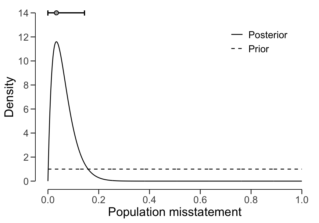
The likelihood

The likelihood function measures the plausibility of the data given different possible values of the misstatement rate. In other words, it quantifies how well the data align with the possible values of the misstatement rate. Suppose you review an audit sample where you find 1 misstatement in 30 items. In this example, the likelihood function measures for all possible misstatement rates how plausible it is to discover 1 misstatement in 30 items.

The posterior distribution

The posterior distribution (or just the posterior) is the result of the Bayesian inference process. It combines the prior information and the likelihood of the data into an updated probability distribution for the misstatement rate. The posterior is often summarized by giving a point estimate (in auditing this is often the mode of the posterior distribution) and an interval estimate (like a 95 percent credible interval). The 95 percent credible interval represents the values between which, with 95 percent probability, the misstatement rate lies.

The solid line in the first image above shows the posterior distribution that results from the uniform prior distribution and a sample of 30 items containing 1 misstatement. The one-sided 95 percent credible interval above the distribution shows the most likely misstatement rate (\(\frac{1}{30}\) = 0.033, or 3.33 percent) and the 95 percent upper bound, which is represented by the right side of the interval and lies around 14.4 percent.

The solid line in the second image shows the posterior distribution using a beta(\(\alpha\) = 1, \(\beta\) = 20) prior. Under this posterior distribution, the 95 percent upper bound is around 9.1 percent, which is 5.3 percent lower than the same upper bound under the other posterior. Hence, incorporating information into the prior distribution can result in a more efficient sample evaluation because less samples are required to achieve a certain amount of assurance.

R code

The images above can be recreated using the following R code, which uses the jfa package for statistical auditing.

R code

Welcome to the very first post on the brand-new 'Blog' page at statisticalauditing.com. Going forward, this page will contain informal discussions from our team members about all things statistical auditing. We are planning to write a short post every week, so stay tuned.

Happy reading!